Premise
The CAPM definition of Beta and Pearson’s correlation coefficient are based on the statistical model of linear regression using the least squares method. This model is perfectly appropriate for measuring the relationship between two returns in a simple way. The vulnerability comes from the use of the whole return series to measure Beta and correlation for financial returns. The linear regression with least squares method is very sensitive to outliers – the kinds of outliers we find frequently in finance because of the complex and unstable interactions of market factors.
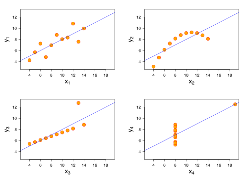
The diagram to the right is taken from Wikipedia (http://en.wikipedia.org/wiki/Anscombe’s_quartet) and shows four distributions with exactly the same Betas and correlations. None of us would feel comfortable saying that these distributions are equally well-described by the regression model.
Capital Risk and Performance Risk
Outliers are a fact of life in the financial markets. These so-called “Black Swan” events occur more frequently than expected and they are a particularly relevant issue in any discussion of risk management, capital adequacy and systemic risk in the global financial system since the new millennium. It is my opinion that these events, as important as they are, need to be distinguished from the expected range of events.
I distinguish between “Capital Risk” and “Performance Risk”.
- Performance Risk is the expected uncertainty of outcomes we manage as a part of our business model. Our business models, which include our portfolios as well as our investment management firms, are designed and built to manage this level of uncertainty. There may be pain – staffing cuts, investor redemptions, lower fees – but this is a performance issue.
- Capital Risk is the risk of capital sufficiency outside an on-going business model assumption. Now we are scrambling to raise capital, negotiating with creditors and gating our funds. These two levels of risk are managed in different ways, including, ultimately, by our governments.
Much of the discussion of the recent financial crisis (and the promotion of “Black Swans”) has been due to a confusion of these two levels of risk and the appropriate mechanism for measuring and managing them. This confusion is not new:
- Annualized Volatility is the most frequently used measure of risk, yet it is calibrated to include only an expected 68.27% of the returns. The other 31.73% still exists but is not used as the basis for analysis and allocation of a portfolio.
- Value-at-Risk is a probabilistic measure of the uncertainty of loss at a pre-defined acceptance level – typically 95% or 99%. Greater losses will happen more frequently than we expect and with greater severity than we expect from this VaR model, but that is not a flaw in the model.
These models are designed to measure and manage the Performance Risk of an on-going business assumption. The remaining risk, Capital Risk, is due to different processes and is managed by different mechanisms. We create portfolios that we expect to perform well under conditions that we expect to experience. We cannot create all our portfolios in expectation of a continuously imminent Black Swan event. Just as we calibrate Annualized Volatility and Value-at-Risk to a given level of expectations, so we should calibrate Alpha, Beta, Correlation and R2 to conform to expectations rather than the whole sample.
Partial Natural Beta and Correlation
Unfortunately, the linear regression model underpinning Beta and correlation uses 100% of the returns and is particularly sensitive (due to least squares) to the outlier events. Not a good combination for measures that we use to allocate capital and measure risk as a part of the on-going business assumption. Looking at the four examples above makes one wonder if there is a better way! There is and without adding a lot of conceptual or practical complexity.

The chart above shows the linear regression relationship between the S&P 500 returns and the HFRI Macro returns taken from the Partial Natural Beta and Correlation example workbook. The results in blue include the three red outliers and show a Beta of 0.0576 with an R2 of only 0.0225 – an insignificant relationship. The results in red show the Partial Natural Beta of 0.1889 with an R2 of 0.1509. Removal of the red outliers (95% of the sample) but keeping the same linear regression model has changed the relationship to a higher Beta with a stronger R2.
Is one more correct than the other? No. The traditional Beta includes the outliers and shows a weak measure for the relationship between HFRI Macro and S&P 500. The stronger measure from Partial Natural Beta shows the ‘effective’ Beta we would expect 95% of the time. In most cases our portfolio risk is that we will experience asset Betas in excess of the expected Betas. In that case we should be measuring the ‘effective’ Beta that shows how high the expected Beta could be 95% or 99% of the time.
Why This Matters
Most of the descriptive statistics that are used for investment analysis were developed for other fields and may not be relevant for the way in which we want to apply them. The problem is that these statistics provide a lingua franca between people, even those who may not understand the details. This, in my opinion, is especially true of investment correlation and Beta. These are fundamental tools we need, but not at the cost of numbers that do not represent the core relationships.
Partial Natural Beta and Partial Natural Correlation use the standard linear regression with least squares method for estimating Beta and Pearson’s correlation, but in a different way. Within any given sample (daily or monthly returns, for example) the most extreme events are excluded to retain the expected events at both the 95% and 99% acceptance levels – Partial. These expected events are then used to estimate the Beta and Pearson’s correlation with the standard calculations – Natural. The result is a more functional measure of these important parameters. They now measure the ‘effective’ relationships we expect most of the time without the excess sensitivity to the extreme events.